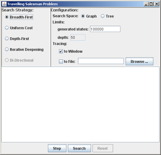
Figure 1: The window of the application
The travelling salesman problem is a classic problem in computer science that can be defined as follows (see also Wikipedia):
Given a number of cities and the costs of travelling from any city to any other city, find the least-cost round-trip route that visits each city exactly once and then returns to the starting city.
This problem can be solved by search. To set it up as a search problem, the initial state is simply the path consisting of the starting city only. Successor states lengthen a given path by one city to which there must be a route and which is not on the path yet. Finally, the goal state is a complete round trip.
TravellingSalesmanApp is a Java application that explores the above search space using a number of (uninformed) search strategies. Download the application and double-click it. Alternatively, run the command "java -jar TravellingSalesmanApp.jar" from the command line. Either should bring up a window that looks essentially like the one shown in figure 1.
Figure 1: The window of the application
To search for a solution, first select a search strategy. Bi-directional search is not available as there is no unique known goal state. Next, there are some configuration options for the search process. If the search space is to be searched as a graph, multiple paths leading to the same node will usually only be explored once. In a tree, search states that can be reached by multiple paths will also be explored multiple times. The number of states to be generated can be limited to the given value, resulting in the search being abandoned at that point. For a depth-first search it is also possible to set a depth limit, meaning no states at a greater depth will be explored.
When the Step or Search button is used to start the search process a dialog comes up in which a file defining the cities and the distances between them has to be selected.
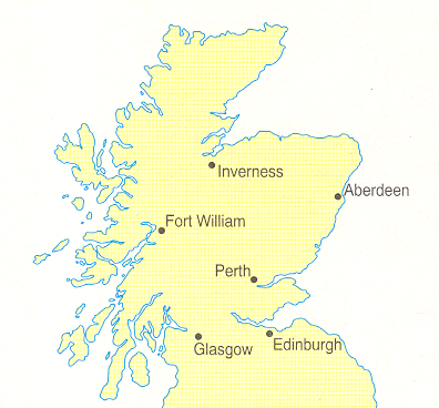 The expected file must be in CSV format which can be created using MS Excel, or any text editor. The format of the file is as follows: each line contains the names of two cities that are connected and the distance between them. For example, a round trip in Scotland involving the cities shown on the map on the right could be specified in a file containing:
Edinburgh,Glasgow,47.0
Edinburgh,Perth,42.0
Glasgow,Perth,61.0
Glasgow,Fort William,102.0
Perth,Fort William,102.0
Perth,Inverness,114.0
Perth,Aberdeen,86.0
Fort William,Inverness,65.0
Fort William,Aberdeen,156.0
Inverness,Aberdeen,106.0
The first city in the first line is taken as the starting and end point for the round trip. Selecting the problem file immediately starts the search. A trace of the search can be written to the window and/or a text file. The operation performed by a search engine consists of selecting a current search node and generating its successors, and the trace reflects this process. For example, the line:
current state: 2: <State : 0-1>
indicates that the selected node contains the given state. The number (2 in the example) is the unique identifier for the search node. Note that there may be multiple nodes that contain the same state, especially when tree search is performed. Then there is a description of the selected state which represents a partial round trip, here starting from city 0 and travelling to city 1. Numbers are assigned in the order in which city names appear in the file describing the problem. Here, 0 represents Edinburgh and 1 represents Glasgow, 2 represents Perth, and so on. The lines following this one in the trace describe the successor states that have been generated, for example:
successor state: 7: <State : 0-1-3>
successor state: 8: <State : 0-1-2>
So, expanding the given search node (2) resulted in two new search nodes (7 and 8), travelling on from Glasgow to Fort William or to Perth.
Even with tracing off the window will display some information about the search (which is not part of the trace). It will show how many states have been explored (the goal test has been performed and successors have been generated) and how many states have been generated (explored states plus fringe nodes). If a solution is found this will also be printed. Finally, the elapsed time taken to perform the search is printed. Note that writing the trace usually takes more time than searching itself.
S. Russell and P. Norvig. Artificial Intelligence: A Modern Approach, chapter 3. Prentice Hall, 2nd edition, 2003.